« Previous
Next »
« Previous
Next »
MICROSOFT EXCEL 2013
Lookup & Reference:
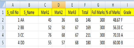
- VLOOKUP() Searches for a value in the first column of a table array and returns a value in the same row from another column in the table array.
- First Type the below data in Sheet1 as below format.
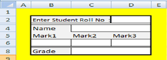
- Type the below format in sheet 2 of your same work book.
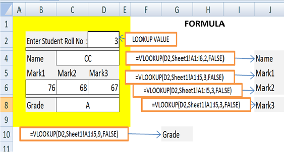
- Type the formula for Name, Mark1, Mark2, Mark3 and Grade in the Cell C4, B6, C6, D6 and C8 respectively.
- Enter the Roll No in D2 cell to display the result as above.
Syntax VLOOKUP(lookup_value,table_array,col_index_num,range_lookup)
Lookup_value The value to search in the first column of the table .Lookup_value can be a value or a reference. If lookup_value is smaller than the smallest value in the first column of table_array, VLOOKUP returns the #N/A error value. Table_array Two or more columns of data. Use a reference to a range or a range name. The values in the first column of table_array are the values searched by lookup_value. These values can be text, numbers, or logical values. Uppercase and lowercase text are equivalent. Col_index_num The column number in table_array from which the matching value must be returned. A col_index_num of 1 returns the value in the first column in table_array; a col_index_num of 2 returns the value in the second column in table_array, and so on. If col_index_num is:Less than 1, VLOOKUP returns the #VALUE! error value. Greater than the number of columns in table_array, VLOOKUP returns the #REF! error value. Range_lookup A logicalvalue (true/false) that specifies whether you want VLOOKUP to find an exact match or an approximate match: If TRUE or omitted, an exact or approximate match is returned. If an exact match is not found, the next largest value that is less than lookup_value is returned. The values in the first column of table_array must be placed in ascending sort order; otherwise, VLOOKUP may not give the correct value. If FALSE, VLOOKUP will only find an exact match. In this case, the values in the first column of table_array do not need to be sorted. If there are two or more values in the first column of table_array that match the lookup_value, the first value found is used. If an exact match is not found, the error value #N/A is returned. Ex: This example searches name, mark of 3subjects and grade by entering roll number from a student marks data tables.